Application Developer Guide
The Apex platform is designed to process massive amounts of real-time events natively in Hadoop. It runs as a YARN (Hadoop 2.x) application and leverages Hadoop as a distributed operating system. All the basic distributed operating system capabilities of Hadoop like resource management (YARN), distributed file system (HDFS), multi-tenancy, security, fault-tolerance, and scalability are supported natively in all the Apex applications. The platform handles all the details of the application execution, including dynamic scaling, state checkpointing and recovery, event processing guarantees, etc. allowing you to focus on writing your application logic without mixing operational and functional concerns.
In the platform, building a streaming application can be extremely easy and intuitive. The application is represented as a Directed Acyclic Graph (DAG) of computation units called Operators interconnected by the data-flow edges called Streams. The operators process input streams and produce output streams. A library of common operators is provided to enable quick application development. In case the desired processing is not available in the Operator Library, one can easily write a custom operator. We refer those interested in creating their own operators to the Operator Development Guide.
Running A Test Application
If you are starting with the Apex platform for the first time, it can be informative to launch an existing application and see it run. One of the simplest examples provided in Apex-Malhar repository is a Pi demo application, which computes the value of PI using random numbers. After setting up development environment Pi demo can be launched as follows:
- Open up Apex Malhar files in your IDE (for example Eclipse, IntelliJ, NetBeans, etc)
- Navigate to
demos/pi/src/test/java/com/datatorrent/demos/ApplicationTest.java - Run the test for ApplicationTest.java
- View the output in system console
Congratulations, you just ran your first real-time streaming demo :) This demo is very simple and has four operators. The first operator emits random integers between 0 to 30, 000. The second operator receives these coefficients and emits a hashmap with x and y values each time it receives two values. The third operator takes these values and computes x**2+y**2. The last operator counts how many computed values from the previous operator were less than or equal to 30, 000**2. Assuming this count is N, then PI is computed as N/number of values received. Here is the code snippet for the PI application. This code populates the DAG. Do not worry about what each line does, we will cover these concepts later in this document.
// Generates random numbers
RandomEventGenerator rand = dag.addOperator("rand", new RandomEventGenerator());
rand.setMinvalue(0);
rand.setMaxvalue(30000);

// Generates a round robin HashMap of "x" and "y"
RoundRobinHashMap<String,Object> rrhm = dag.addOperator("rrhm", new RoundRobinHashMap<String, Object>());
rrhm.setKeys(new String[] { "x", "y" });

// Calculates pi from x and y
JavaScriptOperator calc = dag.addOperator("picalc", new Script());
calc.setPassThru(false);
calc.put("i",0);
calc.put("count",0);
calc.addSetupScript("function pi() { if (x*x+y*y <= "+maxValue*maxValue+") { i++; } count++; return i / count * 4; }");
calc.setInvoke("pi");
dag.addStream("rand_rrhm", rand.integer_data, rrhm.data);
dag.addStream("rrhm_calc", rrhm.map, calc.inBindings);

// puts results on system console
ConsoleOutputOperator console = dag.addOperator("console", new ConsoleOutputOperator());
dag.addStream("rand_console",calc.result, console.input);
You can review the other demos and see what they do. The examples given in the Demos project cover various features of the platform and we strongly encourage you to read these to familiarize yourself with the platform. In the remaining part of this document we will go through details needed for you to develop and run streaming applications in Malhar.
Test Application: Yahoo! Finance Quotes
The PI application was to get you started. It is a basic application and does not fully illustrate the features of the platform. For the purpose of describing concepts, we will consider the test application shown in Figure 1. The application downloads tick data from Yahoo! Finance and computes the following for four tickers, namely IBM, GOOG, YHOO.
- Quote: Consisting of last trade price, last trade time, and total volume for the day
- Per-minute chart data: Highest trade price, lowest trade price, and volume during that minute
- Simple Moving Average: trade price over 5 minutes
Total volume must ensure that all trade volume for that day is added, i.e. data loss would result in wrong results. Charting data needs all the trades in the same minute to go to the same slot, and then on it starts afresh, so again data loss would result in wrong results. The aggregation for charting data is done over 1 minute. Simple moving average computes the average price over a 5 minute sliding window; it too would produce wrong results if there is data loss. Figure 1 shows the application with no partitioning.
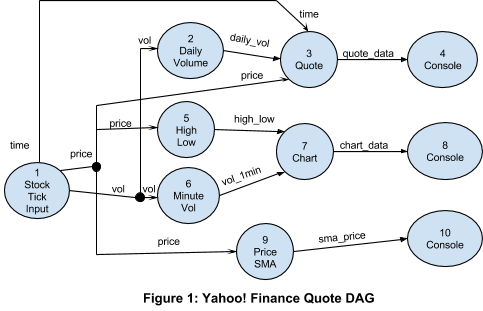
The operator StockTickerInput: StockTickerInput is the input operator that reads live data from Yahoo! Finance once per interval (user configurable in milliseconds), and emits the price, the incremental volume, and the last trade time of each stock symbol, thus emulating real ticks from the exchange. We utilize the Yahoo! Finance CSV web service interface. For example:
$ GET 'http://download.finance.yahoo.com/d/quotes.csv?s=IBM,GOOG,AAPL,YHOO&f=sl1vt1'
"IBM",203.966,1513041,"1:43pm"
"GOOG",762.68,1879741,"1:43pm"
"AAPL",444.3385,11738366,"1:43pm"
"YHOO",19.3681,14707163,"1:43pm"
Among all the operators in Figure 1, StockTickerInput is the only operator that requires extra code because it contains a custom mechanism to get the input data. Other operators are used unchanged from the Malhar library.
Here is the class implementation for StockTickInput:
package com.datatorrent.demos.yahoofinance;

import au.com.bytecode.opencsv.CSVReader;
import com.datatorrent.annotation.OutputPortFieldAnnotation;
import com.datatorrent.api.Context.OperatorContext;
import com.datatorrent.api.DefaultOutputPort;
import com.datatorrent.api.InputOperator;
import com.datatorrent.lib.util.KeyValPair;
import java.io.IOException;
import java.io.InputStream;
import java.io.InputStreamReader;
import java.util.*;
import org.apache.commons.httpclient.HttpClient;
import org.apache.commons.httpclient.HttpStatus;
import org.apache.commons.httpclient.cookie.CookiePolicy;
import org.apache.commons.httpclient.methods.GetMethod;
import org.apache.commons.httpclient.params.DefaultHttpParams;
import org.slf4j.Logger;
import org.slf4j.LoggerFactory;

/**
 * This operator sends price, volume and time into separate ports and calculates incremental volume.
 */
public class StockTickInput implements InputOperator
{
  private static final Logger logger = LoggerFactory.getLogger(StockTickInput.class);
  /**
   * Timeout interval for reading from server. 0 or negative indicates no timeout.
   */
  public int readIntervalMillis = 500;
  /**
   * The URL of the web service resource for the POST request.
   */
  private String url;
  public String[] symbols;
  private transient HttpClient client;
  private transient GetMethod method;
  private HashMap<String, Long> lastVolume = new HashMap<String, Long>();
  private boolean outputEvenIfZeroVolume = false;
  /**
   * The output port to emit price.
   */
  @OutputPortFieldAnnotation(optional = true)
  public final transient DefaultOutputPort<KeyValPair<String, Double>> price = new DefaultOutputPort<KeyValPair<String, Double>>();
  /**
   * The output port to emit incremental volume.
   */
  @OutputPortFieldAnnotation(optional = true)
  public final transient DefaultOutputPort<KeyValPair<String, Long>> volume = new DefaultOutputPort<KeyValPair<String, Long>>();
  /**
   * The output port to emit last traded time.
   */
  @OutputPortFieldAnnotation(optional = true)
  public final transient DefaultOutputPort<KeyValPair<String, String>> time = new DefaultOutputPort<KeyValPair<String, String>>();

  /**
   * Prepare URL from symbols and parameters. URL will be something like: http://download.finance.yahoo.com/d/quotes.csv?s=IBM,GOOG,AAPL,YHOO&f=sl1vt1
   *
   * @return the URL
   */
  private String prepareURL()
  {
    String str = "http://download.finance.yahoo.com/d/quotes.csv?s=";
    for (int i = 0; i < symbols.length; i++) {
      if (i != 0) {
        str += ",";
      }
      str += symbols[i];
    }
    str += "&f=sl1vt1&e=.csv";
    return str;
  }

  @Override
  public void setup(OperatorContext context)
  {
    url = prepareURL();
    client = new HttpClient();
    method = new GetMethod(url);
    DefaultHttpParams.getDefaultParams().setParameter("http.protocol.cookie-policy", CookiePolicy.BROWSER_COMPATIBILITY);
  }

  @Override
  public void teardown()
  {
  }

  @Override
  public void emitTuples()
  {

    try {
      int statusCode = client.executeMethod(method);
      if (statusCode != HttpStatus.SC_OK) {
        System.err.println("Method failed: " + method.getStatusLine());
      } else {
        InputStream istream = method.getResponseBodyAsStream();
        // Process response
        InputStreamReader isr = new InputStreamReader(istream);
        CSVReader reader = new CSVReader(isr);
        List<String[]> myEntries = reader.readAll();
        for (String[] stringArr: myEntries) {
          ArrayList<String> tuple = new ArrayList<String>(Arrays.asList(stringArr));
          if (tuple.size() != 4) {
            return;
          }
          // input csv is <Symbol>,<Price>,<Volume>,<Time>
          String symbol = tuple.get(0);
          double currentPrice = Double.valueOf(tuple.get(1));
          long currentVolume = Long.valueOf(tuple.get(2));
          String timeStamp = tuple.get(3);
          long vol = currentVolume;
          // Sends total volume in first tick, and incremental volume afterwards.
          if (lastVolume.containsKey(symbol)) {
            vol -= lastVolume.get(symbol);
          }

          if (vol > 0 || outputEvenIfZeroVolume) {
            price.emit(new KeyValPair<String, Double>(symbol, currentPrice));
            volume.emit(new KeyValPair<String, Long>(symbol, vol));
            time.emit(new KeyValPair<String, String>(symbol, timeStamp));
            lastVolume.put(symbol, currentVolume);
          }
        }
      }
      Thread.sleep(readIntervalMillis);
    } catch (InterruptedException ex) {
      logger.debug(ex.toString());
    } catch (IOException ex) {
      logger.debug(ex.toString());
    }
  }

  @Override
  public void beginWindow(long windowId)
  {
  }

  @Override
  public void endWindow()
  {
  }

  public void setOutputEvenIfZeroVolume(boolean outputEvenIfZeroVolume)
  {
    this.outputEvenIfZeroVolume = outputEvenIfZeroVolume;
  }

}
The operator has three output ports that emit the price of the stock, the volume of the stock and the last trade time of the stock, declared as public member variables price, volume and time of the class. The tuple of the price output port is a key-value pair with the stock symbol being the key, and the price being the value. The tuple of the volume output port is a key value pair with the stock symbol being the key, and the incremental volume being the value. The tuple of the time output port is a key value pair with the stock symbol being the key, and the last trade time being the value.
Important: Since operators will be serialized, all input and output ports need to be declared transient because they are stateless and should not be serialized.
The method setup(OperatorContext) contains the code that is necessary for setting up the HTTP client for querying Yahoo! Finance.
Method emitTuples() contains the code that reads from Yahoo! Finance, and emits the data to the output ports of the operator. emitTuples() will be called one or more times within one application window as long as time is allowed within the window.
Note that we want to emulate the tick input stream by having incremental volume data with Yahoo! Finance data. We therefore subtract the previous volume from the current volume to emulate incremental volume for each tick.
The operator DailyVolume: This operator reads from the input port, which contains the incremental volume tuples from StockTickInput, and aggregates the data to provide the cumulative volume. It uses the library class SumKeyVal<K,V> provided in math package. In this case, SumKeyVal<String,Long>, where K is the stock symbol, V is the aggregated volume, with cumulative set to true. (Otherwise if cumulativewas set to false, SumKeyVal would provide the sum for the application window.) Malhar provides a number of built-in operators for simple operations like this so that application developers do not have to write them. More examples to follow. This operator assumes that the application restarts before the market opens every day.
The operator Quote: This operator has three input ports, which are price (from StockTickInput), daily_vol (from Daily Volume), and time (from StockTickInput). This operator just consolidates the three data items and and emits the consolidated data. It utilizes the class ConsolidatorKeyVal<K> from the stream package.
The operator HighLow: This operator reads from the input port, which contains the price tuples from StockTickInput, and provides the high and the low price within the application window. It utilizes the library class RangeKeyVal<K,V> provided in the math package. In this case, RangeKeyVal<String,Double>.
The operator MinuteVolume: This operator reads from the input port, which contains the volume tuples from StockTickInput, and aggregates the data to provide the sum of the volume within one minute. Like the operator DailyVolume, this operator also uses SumKeyVal<String,Long>, but with cumulative set to false. The Application Window is set to one minute. We will explain how to set this later.
The operator Chart: This operator is very similar to the operator Quote, except that it takes inputs from High Low and Minute Vol and outputs the consolidated tuples to the output port.
The operator PriceSMA: SMA stands for - Simple Moving Average. It reads from the input port, which contains the price tuples from StockTickInput, and provides the moving average price of the stock. It utilizes SimpleMovingAverage<String,Double>, which is provided in the multiwindow package. SimpleMovingAverage keeps track of the data of the previous N application windows in a sliding manner. For each end window event, it provides the average of the data in those application windows.
The operator Console: This operator just outputs the input tuples to the console (or stdout). In this example, there are four console operators, which connect to the output of Quote, Chart, PriceSMA and VolumeSMA. In practice, they should be replaced by operators that use the data to produce visualization artifacts like charts.
Connecting the operators together and constructing the DAG: Now that we know the operators used, we will create the DAG, set the streaming window size, instantiate the operators, and connect the operators together by adding streams that connect the output ports with the input ports among those operators. This code is in the file YahooFinanceApplication.java. Refer to Figure 1 again for the graphical representation of the DAG. The last method in the code, namely getApplication(), does all that. The rest of the methods are just for setting up the operators.
package com.datatorrent.demos.yahoofinance;

import com.datatorrent.api.ApplicationFactory;
import com.datatorrent.api.Context.OperatorContext;
import com.datatorrent.api.DAG;
import com.datatorrent.api.Operator.InputPort;
import com.datatorrent.lib.io.ConsoleOutputOperator;
import com.datatorrent.lib.math.RangeKeyVal;
import com.datatorrent.lib.math.SumKeyVal;
import com.datatorrent.lib.multiwindow.SimpleMovingAverage;
import com.datatorrent.lib.stream.ConsolidatorKeyVal;
import com.datatorrent.lib.util.HighLow;
import org.apache.hadoop.conf.Configuration;

/**
 * Yahoo! Finance application demo. <p>
 *
 * Get Yahoo finance feed and calculate minute price range, minute volume, simple moving average of 5 minutes.
 */
public class Application implements StreamingApplication
{
  private int streamingWindowSizeMilliSeconds = 1000; // 1 second (default is 500ms)
  private int appWindowCountMinute = 60;   // 1 minute
  private int appWindowCountSMA = 5 * 60;  // 5 minute

  /**
   * Get actual Yahoo finance ticks of symbol, last price, total daily volume, and last traded price.
   */
  public StockTickInput getStockTickInputOperator(String name, DAG dag)
  {
    StockTickInput oper = dag.addOperator(name, StockTickInput.class);
    oper.readIntervalMillis = 200;
    return oper;
  }

  /**
   * This sends total daily volume by adding volumes from each ticks.
   */
  public SumKeyVal<String, Long> getDailyVolumeOperator(String name, DAG dag)
  {
    SumKeyVal<String, Long> oper = dag.addOperator(name, new SumKeyVal<String, Long>());
    oper.setType(Long.class);
    oper.setCumulative(true);
    return oper;
  }

  /**
   * Get aggregated volume of 1 minute and send at the end window of 1 minute.
   */
  public SumKeyVal<String, Long> getMinuteVolumeOperator(String name, DAG dag, int appWindowCount)
  {
    SumKeyVal<String, Long> oper = dag.addOperator(name, new SumKeyVal<String, Long>());
    oper.setType(Long.class);
    oper.setEmitOnlyWhenChanged(true);
dag.getOperatorMeta(name).getAttributes().put(OperatorContext.APPLICATION_WINDOW_COUNT,appWindowCount);
    return oper;
  }

  /**
   * Get High-low range for 1 minute.
   */
  public RangeKeyVal<String, Double> getHighLowOperator(String name, DAG dag, int appWindowCount)
  {
    RangeKeyVal<String, Double> oper = dag.addOperator(name, new RangeKeyVal<String, Double>());
    dag.getOperatorMeta(name).getAttributes().put(OperatorContext.APPLICATION_WINDOW_COUNT,appWindowCount);
    oper.setType(Double.class);
    return oper;
  }

  /**
   * Quote (Merge price, daily volume, time)
   */
  public ConsolidatorKeyVal<String,Double,Long,String,?,?> getQuoteOperator(String name, DAG dag)
  {
    ConsolidatorKeyVal<String,Double,Long,String,?,?> oper = dag.addOperator(name, new ConsolidatorKeyVal<String,Double,Long,String,Object,Object>());
    return oper;
  }

  /**
   * Chart (Merge minute volume and minute high-low)
   */
  public ConsolidatorKeyVal<String,HighLow,Long,?,?,?> getChartOperator(String name, DAG dag)
  {
    ConsolidatorKeyVal<String,HighLow,Long,?,?,?> oper = dag.addOperator(name, new ConsolidatorKeyVal<String,HighLow,Long,Object,Object,Object>());
    return oper;
  }

  /**
   * Get simple moving average of price.
   */
  public SimpleMovingAverage<String, Double> getPriceSimpleMovingAverageOperator(String name, DAG dag, int appWindowCount)
  {
    SimpleMovingAverage<String, Double> oper = dag.addOperator(name, new SimpleMovingAverage<String, Double>());
    oper.setWindowSize(appWindowCount);
    oper.setType(Double.class);
    return oper;
  }

  /**
   * Get console for output.
   */
  public InputPort<Object> getConsole(String name, /*String nodeName,*/ DAG dag, String prefix)
  {
    ConsoleOutputOperator oper = dag.addOperator(name, ConsoleOutputOperator.class);
    oper.setStringFormat(prefix + ": %s");
    return oper.input;
  }

  /**
   * Create Yahoo Finance Application DAG.
   */
  @Override
  public void populateDAG(DAG dag, Configuration conf)
  {
    dag.getAttributes().put(DAG.STRAM_WINDOW_SIZE_MILLIS,streamingWindowSizeMilliSeconds);

    StockTickInput tick = getStockTickInputOperator("StockTickInput", dag);
    SumKeyVal<String, Long> dailyVolume = getDailyVolumeOperator("DailyVolume", dag);
    ConsolidatorKeyVal<String,Double,Long,String,?,?> quoteOperator = getQuoteOperator("Quote", dag);

    RangeKeyVal<String, Double> highlow = getHighLowOperator("HighLow", dag, appWindowCountMinute);
    SumKeyVal<String, Long> minuteVolume = getMinuteVolumeOperator("MinuteVolume", dag, appWindowCountMinute);
    ConsolidatorKeyVal<String,HighLow,Long,?,?,?> chartOperator = getChartOperator("Chart", dag);

    SimpleMovingAverage<String, Double> priceSMA = getPriceSimpleMovingAverageOperator("PriceSMA", dag, appWindowCountSMA);
       DefaultPartitionCodec<String, Double> codec = new DefaultPartitionCodec<String, Double>();
    dag.setInputPortAttribute(highlow.data, PortContext.STREAM_CODEC, codec);
    dag.setInputPortAttribute(priceSMA.data, PortContext.STREAM_CODEC, codec);
    dag.addStream("price", tick.price, quoteOperator.in1, highlow.data, priceSMA.data);
    dag.addStream("vol", tick.volume, dailyVolume.data, minuteVolume.data);
    dag.addStream("time", tick.time, quoteOperator.in3);
    dag.addStream("daily_vol", dailyVolume.sum, quoteOperator.in2);

    dag.addStream("quote_data", quoteOperator.out, getConsole("quoteConsole", dag, "QUOTE"));

    dag.addStream("high_low", highlow.range, chartOperator.in1);
    dag.addStream("vol_1min", minuteVolume.sum, chartOperator.in2);
    dag.addStream("chart_data", chartOperator.out, getConsole("chartConsole", dag, "CHART"));

    dag.addStream("sma_price", priceSMA.doubleSMA, getConsole("priceSMAConsole", dag, "Price SMA"));

    return dag;
  }

}
Note that we also set a user-specific sliding window for SMA that keeps track of the previous N data points. Do not confuse this with the attribute APPLICATION_WINDOW_COUNT.
In the rest of this chapter we will run through the process of running this application. We assume that you are familiar with details of your Hadoop infrastructure. For installation details please refer to the Installation Guide.
Running a Test Application
We will now describe how to run the yahoo finance application described above in different modes (local mode, single node on Hadoop, and multi-nodes on Hadoop).
The platform runs streaming applications under the control of a light-weight Streaming Application Manager (STRAM). Each application has its own instance of STRAM. STRAM launches the application and continually provides run time monitoring, analysis, and takes action such as load scaling or outage recovery as needed. We will discuss STRAM in more detail in the next chapter.
The instructions below assume that the platform was installed in a directory <INSTALL_DIR> and the command line interface (CLI) will be used to launch the demo application. An application can be run in local mode (in IDE or from command line) or on a Hadoop cluster.
To start the Apex CLI run
<INSTALL_DIR>/bin/apex
The command line prompt appears. To start the application in local mode (the actual version number in the file name may differ)
apex> launch -local <INSTALL_DIR>/yahoo-finance-demo-3.2.0-SNAPSHOT.apa
To terminate the application in local mode, enter Ctrl-C
Tu run the application on the Hadoop cluster (the actual version number in the file name may differ)
apex> launch <INSTALL_DIR>/yahoo-finance-demo-3.2.0-SNAPSHOT.apa
To stop the application running in Hadoop, terminate it in the Apex CLI:
apex> kill-app
Executing the application in either mode includes the following steps. At a top level, STRAM (Streaming Application Manager) validates the application (DAG), translates the logical plan to the physical plan and then launches the execution engine. The mode determines the resources needed and how how they are used.
Local Mode
In local mode, the application is run as a single-process with multiple threads. Although a few Hadoop classes are needed, there is no dependency on a Hadoop cluster or Hadoop services. The local file system is used in place of HDFS. This mode allows a quick run of an application in a single process sandbox, and hence is the most suitable to debug and analyze the application logic. This mode is recommended for developing the application and can be used for running applications within the IDE for functional testing purposes. Due to limited resources and lack of scalability an application running in this single process mode is more likely to encounter throughput bottlenecks. A distributed cluster is recommended for benchmarking and production testing.
Hadoop Cluster
In this section we discuss various Hadoop cluster setups.
Single Node Cluster
In a single node Hadoop cluster all services are deployed on a single server (a developer can use his/her development machine as a single node cluster). The platform does not distinguish between a single or multi-node setup and behaves exactly the same in both cases.
In this mode, the resource manager, name node, data node, and node manager occupy one process each. This is an example of running a streaming application as a multi-process application on the same server. With prevalence of fast, multi-core systems, this mode is effective for debugging, fine tuning, and generic analysis before submitting the job to a larger Hadoop cluster. In this mode, execution uses the Hadoop services and hence is likely to identify issues that are related to the Hadoop environment (such issues will not be uncovered in local mode). The throughput will obviously not be as high as on a multi-node Hadoop cluster. Additionally, since each container (i.e. Java process) requires a significant amount of memory, you will be able to run a much smaller number of containers than on a multi-node cluster.
Multi-Node Cluster
In a multi-node Hadoop cluster all the services of Hadoop are typically distributed across multiple nodes in a production or production-level test environment. Upon launch the application is submitted to the Hadoop cluster and executes as a multi-processapplication on multiple nodes.
Before you start deploying, testing and troubleshooting your application on a cluster, you should ensure that Hadoop (version 2.6.0 or later) is properly installed and you have basic skills for working with it.
Apache Apex Platform Overview
Streaming Computational Model
In this chapter, we describe the the basics of the real-time streaming platform and its computational model.
The platform is designed to enable completely asynchronous real time computations done in as unblocked a way as possible with minimal overhead .
Applications running in the platform are represented by a Directed Acyclic Graph (DAG) made up of operators and streams. All computations are done in memory on arrival of the input data, with an option to save the output to disk (HDFS) in a non-blocking way. The data that flows between operators consists of atomic data elements. Each data element along with its type definition (henceforth called schema) is called a tuple. An application is a design of the flow of these tuples to and from the appropriate compute units to enable the computation of the final desired results. A message queue (henceforth called buffer server) manages tuples streaming between compute units in different processes.This server keeps track of all consumers, publishers, partitions, and enables replay. More information is given in later section.
The streaming application is monitored by a decision making entity called STRAM (streaming application manager). STRAM is designed to be a light weight controller that has minimal but sufficient interaction with the application. This is done via periodic heartbeats. The STRAM does the initial launch and periodically analyzes the system metrics to decide if any run time action needs to be taken.
A fundamental building block for the streaming platform is the concept of breaking up a stream into equal finite time slices called streaming windows. Each window contains the ordered set of tuples in that time slice. A typical duration of a window is 500 ms, but can be configured per application (the Yahoo! Finance application configures this value in the properties.xml file to be 1000ms = 1s). Each window is preceded by a begin_window event and is terminated by an end_window event, and is assigned a unique window ID. Even though the platform performs computations at the tuple level, bookkeeping is done at the window boundary, making the computations within a window an atomic event in the platform. We can think of each window as an atomic micro-batch of tuples, to be processed together as one atomic operation (See Figure 2).
This atomic batching allows the platform to avoid the very steep per tuple bookkeeping cost and instead has a manageable per batch bookkeeping cost. This translates to higher throughput, low recovery time, and higher scalability. Later in this document we illustrate how the atomic micro-batch concept allows more efficient optimization algorithms.
The platform also has in-built support for application windows. An application window is part of the application specification, and can be a small or large multiple of the streaming window. An example from our Yahoo! Finance test application is the moving average, calculated over a sliding application window of 5 minutes which equates to 300 (= 5 * 60) streaming windows.
Note that these two window concepts are distinct. A streaming window is an abstraction of many tuples into a higher atomic event for easier management. An application window is a group of consecutive streaming windows used for data aggregation (e.g. sum, average, maximum, minimum) on a per operator level.

Alongside the platform, a set of predefined, benchmarked standard library operator templates is provided for ease of use and rapid development of application. These operators are open sourced to Apache Software Foundation under the project name “Malhar” as part of our efforts to foster community innovation. These operators can be used in a DAG as is, while others have properties that can be set to specify the desired computation. Those interested in details, should refer to Apex-Malhar operator library.
The platform is a Hadoop YARN native application. It runs in a Hadoop cluster just like any other YARN application (MapReduce etc.) and is designed to seamlessly integrate with rest of Hadoop technology stack. It leverages Hadoop as much as possible and relies on it as its distributed operating system. Hadoop dependencies include resource management, compute/memory/network allocation, HDFS, security, fault tolerance, monitoring, metrics, multi-tenancy, logging etc. Hadoop classes/concepts are reused as much as possible. The aim is to enable enterprises to leverage their existing Hadoop infrastructure for real time streaming applications. The platform is designed to scale with big data applications and scale with Hadoop.
A streaming application is an asynchronous execution of computations across distributed nodes. All computations are done in parallel on a distributed cluster. The computation model is designed to do as many parallel computations as possible in a non-blocking fashion. The task of monitoring of the entire application is done on (streaming) window boundaries with a streaming window as an atomic entity. A window completion is a quantum of work done. There is no assumption that an operator can be interrupted at precisely a particular tuple or window.
An operator itself also cannot assume or predict the exact time a tuple that it emitted would get consumed by downstream operators. The operator processes the tuples it gets and simply emits new tuples based on its business logic. The only guarantee it has is that the upstream operators are processing either the current or some later window, and the downstream operator is processing either the current or some earlier window. The completion of a window (i.e. propagation of the end_window event through an operator) in any operator guarantees that all upstream operators have finished processing this window. Thus, the end_window event is blocking on an operator with multiple outputs, and is a synchronization point in the DAG. The begin_window event does not have any such restriction, a single begin_window event from any upstream operator triggers the operator to start processing tuples.
Streaming Application Manager (STRAM)
Streaming Application Manager (STRAM) is the Hadoop YARN native application master. STRAM is the first process that is activated upon application launch and orchestrates the streaming application on the platform. STRAM is a lightweight controller process. The responsibilities of STRAM include
-
Running the Application
- Read the logical plan of the application (DAG) submitted by the client
- Validate the logical plan
- Translate the logical plan into a physical plan, where certain operators may be partitioned (i.e. replicated) to multiple operators for handling load.
- Request resources (Hadoop containers) from Resource Manager, per physical plan
- Based on acquired resources and application attributes, create an execution plan by partitioning the DAG into fragments, each assigned to different containers.
- Executes the application by deploying each fragment to its container. Containers then start stream processing and run autonomously, processing one streaming window after another. Each container is represented as an instance of the StreamingContainer class, which updates STRAM via the heartbeat protocol and processes directions received from STRAM.
-
Continually monitoring the application via heartbeats from each StreamingContainer
- Collecting Application System Statistics and Logs
- Logging all application-wide decisions taken
- Providing system data on the state of the application via a Web Service.
-
Supporting Fault Tolerance
a. Detecting a node outage b. Requesting a replacement resource from the Resource Manager and scheduling state restoration for the streaming operators c. Saving state to Zookeeper
-
Supporting Dynamic Partitioning: Periodically evaluating the SLA and modifying the physical plan if required (logical plan does not change).
- Enabling Security: Distributing security tokens for distributed components of the execution engine and securing web service requests.
- Enabling Dynamic modification of DAG: In the future, we intend to allow for user initiated modification of the logical plan to allow for changes to the processing logic and functionality.
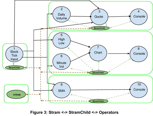
An example of the Yahoo! Finance Quote application scheduled on a cluster of 5 Hadoop containers (processes) is shown in Figure 3.
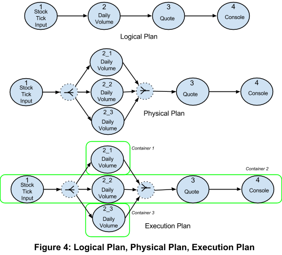
An example for the translation from a logical plan to a physical plan and an execution plan for a subset of the application is shown in Figure 4.
Hadoop Components
In this section we cover some aspects of Hadoop that your streaming application interacts with. This section is not meant to educate the reader on Hadoop, but just get the reader acquainted with the terms. We strongly advise readers to learn Hadoop from other sources.
A streaming application runs as a native Hadoop 2.x application. Hadoop 2.x does not differentiate between a map-reduce job and other applications, and hence as far as Hadoop is concerned, the streaming application is just another job. This means that your application leverages all the bells and whistles Hadoop provides and is fully supported within Hadoop technology stack. The platform is responsible for properly integrating itself with the relevant components of Hadoop that exist today and those that may emerge in the future
All investments that leverage multi-tenancy (for example quotas and queues), security (for example kerberos), data flow integration (for example copying data in-out of HDFS), monitoring, metrics collections, etc. will require no changes when streaming applications run on Hadoop.
YARN
YARNis the core library of Hadoop 2.x that is tasked with resource management and works as a distributed application framework. In this section we will walk through Yarn's components. In Hadoop 2.x, the old jobTracker has been replaced by a combination of ResourceManager (RM) and ApplicationMaster (AM).
Resource Manager (RM)
ResourceManager(RM) manages all the distributed resources. It allocates and arbitrates all the slots and the resources (cpu, memory, network) of these slots. It works with per-node NodeManagers (NMs) and per-application ApplicationMasters (AMs). Currently memory usage is monitored by RM; in upcoming releases it will have CPU as well as network management. RM is shared by map-reduce and streaming applications. Running streaming applications requires no changes in the RM.
Application Master (AM)
The AM is the watchdog or monitoring process for your application and has the responsibility of negotiating resources with RM and interacting with NodeManagers to get the allocated containers started. The AM is the starting point of your application and is considered user code (not system Hadoop code). The AM itself runs in one container. All resource management within the application are managed by the AM. This is a critical feature for Hadoop 2.x where tasks done by jobTracker in Hadoop 1.0 have been distributed allowing Hadoop 2.x to scale much beyond Hadoop 1.0. STRAM is a native YARN ApplicationManager.
Node Managers (NM)
There is one NodeManager(NM) per node in the cluster. All the containers (i.e. processes) on that node are monitored by the NM. It takes instructions from RM and manages resources of that node as per RM instructions. NMs interactions are same for map-reduce and for streaming applications. Running streaming applications requires no changes in the NM.
RPC Protocol
Communication among RM, AM, and NM is done via the Hadoop RPC protocol. Streaming applications use the same protocol to send their data. No changes are needed in RPC support provided by Hadoop to enable communication done by components of your application.
HDFS
Hadoop includes a highly fault tolerant, high throughput distributed file system (HDFS). It runs on commodity hardware, and your streaming application will, by default, use it. There is no difference between files created by a streaming application and those created by map-reduce.
Developing An Application
In this chapter we describe the methodology to develop an application using the Realtime Streaming Platform. The platform was designed to make it easy to build and launch sophisticated streaming applications with the developer having to deal only with the application/business logic. The platform deals with details of where to run what operators on which servers and how to correctly route streams of data among them.
Development Process
While the platform does not mandate a specific methodology or set of development tools, we have recommendations to maximize productivity for the different phases of application development.
Design
- Identify common, reusable operators. Use a library if possible.
- Identify scalability and performance requirements before designing the DAG.
- Leverage attributes that the platform supports for scalability and performance.
- Use operators that are benchmarked and tested so that later surprises are minimized. If you have glue code, create appropriate unit tests for it.
- Use THREAD_LOCAL locality for high throughput streams. If all the operators on that stream cannot fit in one container, try NODE_LOCAL locality. Both THREAD_LOCAL and NODE_LOCAL streams avoid the Network Interface Card (NIC) completly. The former uses intra-process communication to also avoid serialization-deserialization overhead.
- The overall throughput and latencies are are not necessarily correlated to the number of operators in a simple way -- the relationship is more nuanced. A lot depends on how much work individual operators are doing, how many are able to operate in parallel, and how much data is flowing through the arcs of the DAG. It is, at times, better to break a computation down into its constituent simple parts and then stitch them together via streams to better utilize the compute resources of the cluster. Decide on a per application basis the fine line between complexity of each operator vs too many streams. Doing multiple computations in one operator does save network I/O, while operators that are too complex are hard to maintain.
- Do not use operators that depend on the order of two streams as far as possible. In such cases behavior is not idempotent.
- Persist key information to HDFS if possible; it may be useful for debugging later.
- Decide on an appropriate fault tolerance mechanism. If some data loss is acceptable, use the at-most-once mechanism as it has fastest recovery.
Creating New Project
Please refer to the Apex Application Packages for the basic steps for creating a new project.
Writing the application code
Preferably use an IDE (Eclipse, Netbeans etc.) that allows you to manage dependencies and assists with the Java coding. Specific benefits include ease of managing operator library jar files, individual operator classes, ports and properties. It will also highlight and assist to rectify issues such as type mismatches when adding streams while typing.
Testing
Write test cases with JUnit or similar test framework so that code is tested as it is written. For such testing, the DAG can run in local mode within the IDE. Doing this may involve writing mock input or output operators for the integration points with external systems. For example, instead of reading from a live data stream, the application in test mode can read from and write to files. This can be done with a single application DAG by instrumenting a test mode using settings in the configuration that is passed to the application factory interface.
Good test coverage will not only eliminate basic validation errors such as missing port connections or property constraint violations, but also validate the correct processing of the data. The same tests can be re-run whenever the application or its dependencies change (operator libraries, version of the platform etc.)
Running an application
The platform provides a commandline tool called apex for managing applications (launching, killing, viewing, etc.). This tool was already discussed above briefly in the section entitled Running the Test Application. It will introspect the jar file specified with the launch command for applications (classes that implement ApplicationFactory) or properties files that define applications. It will also deploy the dependency jar files from the application package to the cluster.
Apex CLI can run the application in local mode (i.e. outside a cluster). It is recommended to first run the application in local mode in the development environment before launching on the Hadoop cluster. This way some of the external system integration and correct functionality of the application can be verified in an easier to debug environment before testing distributed mode.
For more details on CLI please refer to the Apex CLI Guide.
Application API
This section introduces the API to write a streaming application. The work involves connecting operators via streams to form the logical DAG. The steps are
-
Instantiate an application (DAG)
-
(Optional) Set Attributes
- Assign application name
- Set any other attributes as per application requirements
-
Create/re-use and instantiate operators
- Assign operator name that is unique within the application
- Declare schema upfront for each operator (and thereby its ports)
- (Optional) Set properties and attributes on the dag as per specification
- Connect ports of operators via streams
- Each stream connects one output port of an operator to one or more input ports of other operators.
- (Optional) Set attributes on the streams
-
Test the application.
There are two methods to create an application, namely Java, and Properties file. Java API is for applications being developed by humans, and properties file (Hadoop like) is more suited for DAGs generated by tools.
Java API
The Java API is the most common way to create a streaming application. It is meant for application developers who prefer to leverage the features of Java, and the ease of use and enhanced productivity provided by IDEs like NetBeans or Eclipse. Using Java to specify the application provides extra validation abilities of Java compiler, such as compile time checks for type safety at the time of writing the code. Later in this chapter you can read more about validation support in the platform.
The developer specifies the streaming application by implementing the ApplicationFactory interface, which is how platform tools (CLI etc.) recognize and instantiate applications. Here we show how to create a Yahoo! Finance application that streams the last trade price of a ticker and computes the high and low price in every 1 min window. Run above test application to execute the DAG in local mode within the IDE.
Let us revisit how the Yahoo! Finance test application constructs the DAG:
public class Application implements StreamingApplication
{

  ...

  @Override
  public void populateDAG(DAG dag, Configuration conf)
  {
    dag.getAttributes().attr(DAG.STRAM_WINDOW_SIZE_MILLIS).set(streamingWindowSizeMilliSeconds);

    StockTickInput tick = getStockTickInputOperator("StockTickInput", dag);
    SumKeyVal<String, Long> dailyVolume = getDailyVolumeOperator("DailyVolume", dag);
    ConsolidatorKeyVal<String,Double,Long,String,?,?> quoteOperator = getQuoteOperator("Quote", dag);

    RangeKeyVal<String, Double> highlow = getHighLowOperator("HighLow", dag, appWindowCountMinute);
    SumKeyVal<String, Long> minuteVolume = getMinuteVolumeOperator("MinuteVolume", dag, appWindowCountMinute);
    ConsolidatorKeyVal<String,HighLow,Long,?,?,?> chartOperator = getChartOperator("Chart", dag);

    SimpleMovingAverage<String, Double> priceSMA = getPriceSimpleMovingAverageOperator("PriceSMA", dag, appWindowCountSMA);

    dag.addStream("price", tick.price, quoteOperator.in1, highlow.data, priceSMA.data);
    dag.addStream("vol", tick.volume, dailyVolume.data, minuteVolume.data);
    dag.addStream("time", tick.time, quoteOperator.in3);
    dag.addStream("daily_vol", dailyVolume.sum, quoteOperator.in2);

    dag.addStream("quote_data", quoteOperator.out, getConsole("quoteConsole", dag, "QUOTE"));

    dag.addStream("high_low", highlow.range, chartOperator.in1);
    dag.addStream("vol_1min", minuteVolume.sum, chartOperator.in2);
    dag.addStream("chart_data", chartOperator.out, getConsole("chartConsole", dag, "CHART"));

    dag.addStream("sma_price", priceSMA.doubleSMA, getConsole("priceSMAConsole", dag, "Price SMA"));

    return dag;
  }
}
JSON File DAG Specification
In addition to Java, you can also specify the DAG using JSON, provided the operators in the DAG are present in the dependency jars. Create src/main/resources/app directory under your app package project, and put your JSON files there. This is the specification of a JSON file that specifies an application.
Create a json file under src/main/resources/app, For example myApplication.json
{
  "description": "{application description}",
  "operators": [
    {
      "name": "{operator name}",
      "class": "{fully qualified class name of the operator}",
      "properties": {
        "{property key}": "{property value}",
        ...
      }
    }, ...
  ],
  "streams": [
    {
      "name": "{stream name}",
      "source": {
        "operatorName": "{source operator name}",
        "portName": "{source operator output port name}"
      }
      "sinks": [
        {
          "operatorName": "{sink operator name}",
          "portName": "{sink operator input port name}"
        }, ...
      ]
    }, ...
  ]
}
- The name of the JSON file is taken as the name of the application.
- The
descriptionfield is the description of the application and is optional. - The
operatorsfield is the list of operators the application has. You can specifiy the name, the Java class, and the properties of each operator here. - The
streamsfield is the list of streams that connects the operators together to form the DAG. Each stream consists of the stream name, the operator and port that it connects from, and the list of operators and ports that it connects to. Note that you can connect from one output port of an operator to multiple different input ports of different operators.
In Apex Malhar, there is an example in the Pi Demo doing just that.
Properties File DAG Specification
The platform also supports specification of a DAG via a properties file. The aim here to make it easy for tools to create and run an application. This method of specification does not have the Java compiler support of compile time check, but since these applications would be created by software, they should be correct by construction. The syntax is derived from Hadoop properties and should be easy for folks who are used to creating software that integrated with Hadoop.
Under the src/main/resources/app directory (create if it doesn't exist), create a properties file.
For example myApplication.properties
# input operator that reads from a file
apex.operator.inputOp.classname=com.acme.SampleInputOperator
apex.operator.inputOp.fileName=somefile.txt

# output operator that writes to the console
apex.operator.outputOp.classname=com.acme.ConsoleOutputOperator

# stream connecting both operators
apex.stream.inputStream.source=inputOp.outputPort
apex.stream.inputStream.sinks=outputOp.inputPort
Above snippet is intended to convey the basic idea of specifying the DAG using properties file. Operators would come from a predefined library and referenced in the specification by class name and port names (obtained from the library providers documentation or runtime introspection by tools). For those interested in details, see later sections and refer to the Operation and Installation Guide mentioned above.
Attributes
Attributes impact the runtime behavior of the application. They do not impact the functionality. An example of an attribute is application name. Setting it changes the application name. Another example is streaming window size. Setting it changes the streaming window size from the default value to the specified value. Users cannot add new attributes, they can only choose from the ones that come packaged and pre-supported by the platform. Details of attributes are covered in the Operation and Installation Guide.
Operators
Operators are basic compute units. Operators process each incoming tuple and emit zero or more tuples on output ports as per the business logic. The data flow, connectivity, fault tolerance (node outage), etc. is taken care of by the platform. As an operator developer, all that is needed is to figure out what to do with the incoming tuple and when (and which output port) to send out a particular output tuple. Correctly designed operators will most likely get reused. Operator design needs care and foresight. For details, refer to the Operator Developer Guide. As an application developer you need to connect operators in a way that it implements your business logic. You may also require operator customization for functionality and use attributes for performance/scalability etc.
All operators process tuples asynchronously in a distributed cluster. An operator cannot assume or predict the exact time a tuple that it emitted will get consumed by a downstream operator. An operator also cannot predict the exact time when a tuple arrives from an upstream operator. The only guarantee is that the upstream operators are processing the current or a future window, i.e. the windowId of upstream operator is equals or exceeds its own windowId. Conversely the windowId of a downstream operator is less than or equals its own windowId. The end of a window operation, i.e. the API call to endWindow on an operator requires that all upstream operators have finished processing this window. This means that completion of processing a window propagates in a blocking fashion through an operator. Later sections provides more details on streams and data flow of tuples.
Each operator has a unique name within the DAG as provided by the user. This is the name of the operator in the logical plan. The name of the operator in the physical plan is an integer assigned to it by STRAM. These integers are use the sequence from 1 to N, where N is total number of physically unique operators in the DAG. Following the same rule, each partitioned instance of a logical operator has its own integer as an id. This id along with the Hadoop container name uniquely identifies the operator in the execution plan of the DAG. The logical names and the physical names are required for web service support. Operators can be accessed via both names. These same names are used while interacting with apex cli to access an operator. Ideally these names should be self-descriptive. For example in Figure 1, the node named “Daily volume” has a physical identifier of 2.
Operator Interface
Operator interface in a DAG consists of ports, properties, and attributes. Operators interact with other components of the DAG via ports. Functional behavior of the operators can be customized via parameters. Run time performance and physical instantiation is controlled by attributes. Ports and parameters are fields (variables) of the Operator class/object, while attributes are meta information that is attached to the operator object via an AttributeMap. An operator must have at least one port. Properties are optional. Attributes are provided by the platform and always have a default value that enables normal functioning of operators.
Ports
Ports are connection points by which an operator receives and emits tuples. These should be transient objects instantiated in the operator object, that implement particular interfaces. Ports should be transient as they contain no state. They have a pre-defined schema and can only be connected to other ports with the same schema. An input port needs to implement the interface Operator.InputPort and interface Sink. A default implementation of these is provided by the abstract class DefaultInputPort. An output port needs to implement the interface Operator.OutputPort. A default implementation of this is provided by the concrete class DefaultOutputPort. These two are a quick way to implement the above interfaces, but operator developers have the option of providing their own implementations.
Here are examples of an input and an output port from the operator Sum.
@InputPortFieldAnnotation(name = "data")
public final transient DefaultInputPort<V> data = new DefaultInputPort<V>() {
  @Override
  public void process(V tuple)
  {
    ...
  }
}
@OutputPortFieldAnnotation(optional=true)
public final transient DefaultOutputPort<V> sum = new DefaultOutputPort<V>(){ … };
The process call is in the Sink interface. An emit on an output port is done via emit(tuple) call. For the above example it would be sum.emit(t), where the type of t is the generic parameter V.
There is no limit on how many ports an operator can have. However any operator must have at least one port. An operator with only one port is called an Input Adapter if it has no input port and an Output Adapter if it has no output port. These are special operators needed to get/read data from outside system/source into the application, or push/write data into an outside system/sink. These could be in Hadoop or outside of Hadoop. These two operators are in essence gateways for the streaming application to communicate with systems outside the application.
Port connectivity can be validated during compile time by adding PortFieldAnnotations shown above. By default all ports have to be connected, to allow a port to go unconnected, you need to add “optional=true” to the annotation.
Attributes can be specified for ports that affect the runtime behavior. An example of an attribute is parallel partition that specifes a parallel computation flow per partition. It is described in detail in the Parallel Partitions section. Another example is queue capacity that specifies the buffer size for the port. Details of attributes are covered in Operation and Installation Guide.
Properties
Properties are the abstractions by which functional behavior of an operator can be customized. They should be non-transient objects instantiated in the operator object. They need to be non-transient since they are part of the operator state and re-construction of the operator object from its checkpointed state must restore the operator to the desired state. Properties are optional, i.e. an operator may or may not have properties; they are part of user code and their values are not interpreted by the platform in any way.
All non-serializable objects should be declared transient. Examples include sockets, session information, etc. These objects should be initialized during setup call, which is called every time the operator is initialized.
Attributes
Attributes are values assigned to the operators that impact run-time. This includes things like the number of partitions, at most once or at least once or exactly once recovery modes, etc. Attributes do not impact functionality of the operator. Users can change certain attributes in runtime. Users cannot add attributes to operators; they are pre-defined by the platform. They are interpreted by the platform and thus cannot be defined in user created code (like properties). Details of attributes are covered in Configuration Guide.
Operator State
The state of an operator is defined as the data that it transfers from one window to a future window. Since the computing model of the platform is to treat windows like micro-batches, the operator state can be checkpointed every Nth window, or every T units of time, where T is significantly greater than the streaming window. When an operator is checkpointed, the entire object is written to HDFS. The larger the amount of state in an operator, the longer it takes to recover from a failure. A stateless operator can recover much quicker than a stateful one. The needed windows are preserved by the upstream buffer server and are used to recompute the lost windows, and also rebuild the buffer server in the current container.
The distinction between Stateless and Stateful is based solely on the need to transfer data in the operator from one window to the next. The state of an operator is independent of the number of ports.
Stateless
A Stateless operator is defined as one where no data is needed to be kept at the end of every window. This means that all the computations of a window can be derived from all the tuples the operator receives within that window. This guarantees that the output of any window can be reconstructed by simply replaying the tuples that arrived in that window. Stateless operators are more efficient in terms of fault tolerance, and cost to achieve SLA.
Stateful
A Stateful operator is defined as one where data is needed to be stored at the end of a window for computations occurring in later window; a common example is the computation of a sum of values in the input tuples.
Operator API
The Operator API consists of methods that operator developers may need to override. In this section we will discuss the Operator APIs from the point of view of an application developer. Knowledge of how an operator works internally is critical for writing an application. Those interested in the details should refer to Malhar Operator Developer Guide.
The APIs are available in three modes, namely Single Streaming Window, Sliding Application Window, and Aggregate Application Window. These are not mutually exclusive, i.e. an operator can use single streaming window as well as sliding application window. A physical instance of an operator is always processing tuples from a single window. The processing of tuples is guaranteed to be sequential, no matter which input port the tuples arrive on.
In the later part of this section we will evaluate three common uses of streaming windows by applications. They have different characteristics and implications on optimization and recovery mechanisms (i.e. algorithm used to recover a node after outage) as discussed later in the section.
Streaming Window
Streaming window is atomic micro-batch computation period. The API methods relating to a streaming window are as follows
public void process(<tuple_type> tuple) // Called on the input port on which the tuple arrives
public void beginWindow(long windowId) // Called at the start of the window as soon as the first begin_window tuple arrives
public void endWindow() // Called at the end of the window after end_window tuples arrive on all input ports
public void setup(OperatorContext context) // Called once during initialization of the operator
public void teardown() // Called once when the operator is being shutdown
A tuple can be emitted in any of the three streaming run-time calls, namely beginWindow, process, and endWindow but not in setup or teardown.
Aggregate Application Window
An operator with an aggregate window is stateful within the application window timeframe and possibly stateless at the end of that application window. An size of an aggregate application window is an operator attribute and is defined as a multiple of the streaming window size. The platform recognizes this attribute and optimizes the operator. The beginWindow, and endWindow calls are not invoked for those streaming windows that do not align with the application window. For example in case of streaming window of 0.5 second and application window of 5 minute, an application window spans 600 streaming windows (5*60*2 = 600). At the start of the sequence of these 600 atomic streaming windows, a beginWindow gets invoked, and at the end of these 600 streaming windows an endWindow gets invoked. All the intermediate streaming windows do not invoke beginWindow or endWindow. Bookkeeping, node recovery, stats, UI, etc. continue to work off streaming windows. For example if operators are being checkpointed say on an average every 30th window, then the above application window would have about 20 checkpoints.
Sliding Application Window
A sliding window is computations that requires previous N streaming windows. After each streaming window the Nth past window is dropped and the new window is added to the computation. An operator with sliding window is a stateful operator at end of any window. The sliding window period is an attribute and is a multiple of streaming window. The platform recognizes this attribute and leverages it during bookkeeping. A sliding aggregate window with tolerance to data loss does not have a very high bookkeeping cost. The cost of all three recovery mechanisms, at most once (data loss tolerant), at least once (data loss intolerant), and exactly once (data loss intolerant and no extra computations) is same as recovery mechanisms based on streaming window. STRAM is not able to leverage this operator for any extra optimization.
Single vs Multi-Input Operator
A single-input operator by definition has a single upstream operator, since there can only be one writing port for a stream. If an operator has a single upstream operator, then the beginWindow on the upstream also blocks the beginWindow of the single-input operator. For an operator to start processing any window at least one upstream operator has to start processing that window. A multi-input operator reads from more than one upstream ports. Such an operator would start processing as soon as the first begin_window event arrives. However the window would not close (i.e. invoke endWindow) till all ports receive end_window events for that windowId. Thus the end of a window is a blocking event. As we saw earlier, a multi-input operator is also the point in the DAG where windows of all upstream operators are synchronized. The windows (atomic micro-batches) from a faster (or just ahead in processing) upstream operators are queued up till the slower upstream operator catches up. STRAM monitors such bottlenecks and takes corrective actions. The platform ensures minimal delay, i.e processing starts as long as at least one upstream operator has started processing.
Recovery Mechanisms
Application developers can set any of the recovery mechanisms below to deal with node outage. In general, the cost of recovery depends on the state of the operator, while data integrity is dependant on the application. The mechanisms are per window as the platform treats windows as atomic compute units. Three recovery mechanisms are supported, namely
- At-least-once: All atomic batches are processed at least once. No data loss occurs.
- At-most-once: All atomic batches are processed at most once. Data loss is possible; this is the most efficient setting.
- Exactly-once: All atomic batches are processed exactly once. No data loss occurs; this is the least efficient setting since additional work is needed to ensure proper semantics.
At-least-once is the default. During a recovery event, the operator connects to the upstream buffer server and asks for windows to be replayed. At-least-once and exactly-once mechanisms start from its checkpointed state. At-most-once starts from the next begin-window event.
Recovery mechanisms can be specified per Operator while writing the application as shown below.
Operator o = dag.addOperator(“operator”, …);
dag.setAttribute(o,  OperatorContext.PROCESSING_MODE,  ProcessingMode.AT_MOST_ONCE);
Also note that once an operator is attributed to AT_MOST_ONCE, all the operators downstream to it have to be AT_MOST_ONCE. The client will give appropriate warnings or errors if that’s not the case.
Details are explained in the chapter on Fault Tolerance below.
Streams
A stream is a connector (edge) abstraction, and is a fundamental building block of the platform. A stream consists of tuples that flow from one port (called the output port) to one or more ports on other operators (called input ports) another -- so note a potentially confusing aspect of this terminology: tuples enter a stream through its output port and leave via one or more input ports. A stream has the following characteristics
- Tuples are always delivered in the same order in which they were emitted.
- Consists of a sequence of windows one after another. Each window being a collection of in-order tuples.
- A stream that connects two containers passes through a buffer server.
- All streams can be persisted (by default in HDFS).
- Exactly one output port writes to the stream.
- Can be read by one or more input ports.
- Connects operators within an application, not outside an application.
- Has an unique name within an application.
- Has attributes which act as hints to STRAM.
-
Streams have four modes, namely in-line, in-node, in-rack, and other. Modes may be overruled (for example due to lack of containers). They are defined as follows:
- THREAD_LOCAL: In the same thread, uses thread stack (intra-thread). This mode can only be used for a downstream operator which has only one input port connected; also called in-line.
- CONTAINER_LOCAL: In the same container (intra-process); also called in-container.
- NODE_LOCAL: In the same Hadoop node (inter processes, skips NIC); also called in-node.
- RACK_LOCAL: On nodes in the same rack; also called in-rack.
- unspecified: No guarantee. Could be anywhere within the cluster
An example of a stream declaration is given below
DAG dag = new DAG();
 …
dag.addStream("views", viewAggregate.sum, cost.data).setLocality(CONTAINER_LOCAL); // A container local  stream
dag.addStream(“clicks”, clickAggregate.sum, rev.data); // An example of unspecified locality
The platform guarantees in-order delivery of tuples in a stream. STRAM views each stream as collection of ordered windows. Since no tuple can exist outside a window, a replay of a stream consists of replay of a set of windows. When multiple input ports read the same stream, the execution plan of a stream ensures that each input port is logically not blocked by the reading of another input port. The schema of a stream is same as the schema of the tuple.
In a stream all tuples emitted by an operator in a window belong to that window. A replay of this window would consists of an in-order replay of all the tuples. Thus the tuple order within a stream is guaranteed. However since an operator may receive multiple streams (for example an operator with two input ports), the order of arrival of two tuples belonging to different streams is not guaranteed. In general in an asynchronous distributed architecture this is expected. Thus the operator (specially one with multiple input ports) should not depend on the tuple order from two streams. One way to cope with this indeterminate order, if necessary, is to wait to get all the tuples of a window and emit results in endWindow call. All operator templates provided as part of Malhar operator library follow these principles.
A logical stream gets partitioned into physical streams each connecting the partition to the upstream operator. If two different attributes are needed on the same stream, it should be split using StreamDuplicator operator.
Modes of the streams are critical for performance. An in-line stream is the most optimal as it simply delivers the tuple as-is without serialization-deserialization. Streams should be marked container_local, specially in case where there is a large tuple volume between two operators which then on drops significantly. Since the setLocality call merely provides a hint, STRAM may ignore it. An In-node stream is not as efficient as an in-line one, but it is clearly better than going off-node since it still avoids the potential bottleneck of the network card.
THREAD_LOCAL and CONTAINER_LOCAL streams do not use a buffer server as this stream is in a single process. The other two do.
Affinity Rules
Affinity Rules in Apex provide a way to specify hints on how operators should be deployed in a cluster. Sometimes you may want to allocate certain operators on the same or different nodes for performance or other reasons. Affinity rules can be used in such cases to make sure these considerations are honored by platform.
There can be two types of rules: Affinity and anti-affinity rules. Affinity rule indicates that the group of operators in the rule should be allocated together. On the other hand, anti-affinity rule indicates that the group of operators should be allocated separately.
Specifying Affinity Rules
A list of Affinity Rules can be specified for an application by setting attribute: DAGContext.AFFINITY_RULES_SET. Here is an example for setting Affinity rules for an application in the populateDag method:
AffinityRulesSet ruleSet = new AffinityRulesSet();
List<AffinityRule> rules = new ArrayList<>();
// Add Affinity rules as per requirement
rules.add(new AffinityRule(Type.ANTI_AFFINITY, Locality.NODE_LOCAL, false, "rand", "operator1", "operator2"));
rules.add(new AffinityRule(Type.AFFINITY, Locality.CONTAINER_LOCAL, false, "console", "rand"));
ruleSet.setAffinityRules(rules);
dag.setAttribute(DAGContext.AFFINITY_RULES_SET, ruleSet);
As shown in the example above, each rule has a type AFFINITY or ANTI_AFFINITY indicating whether operators in the group should be allocated together or separate. These can be applied on any operators in DAG.
The operators for rule can be provided either as a list of 2 or more operator names or as a regular expression. The regex should match at least two operators in DAG to be considered a valid rule. Here is example of rule with regex to allocate all the operators in DAG on the same node:
// Allocate all operators starting with console on same container
rules.add(new AffinityRule(Type.AFFINITY, "*" , Locality.NODE_LOCAL, false));
Likewise, operators for rule can also be added as a list:
// Rule for Operators rand, operator1 and operator2 should not be allocated on same node
rules.add(new AffinityRule(Type.ANTI_AFFINITY, Locality.NODE_LOCAL, false, "rand", "operator1", "operator2"));
To indicate affinity or anti-affinity between partitions of a single operator, list should contain the same operator name twice, as shown in the example below for 'TestOperator'. This will ensure that platform will allocate physical partitions of this operator on different nodes.
// Rule for Partitions of TestOperator should not be allocated on the same node
rules.add(new AffinityRule(Type.ANTI_AFFINITY, Locality.NODE_LOCAL, false, "TestOperator", "TestOperator"));
Another important parameter to indicate affinity rule is the locality constraint. Similar to stream locality, the affinity rule will be applied at either THREAD_LOCAL, CONTAINER_LOCAL or NODE_LOCAL level. Support for RACK_LOCAL is not added yet.
The last configurable parameter for affinity rules is strict or preferred rule. A true value for this parameter indicates that the rule should be relaxed in case sufficient resources are not available.
Specifying affinity rules from properties
The same set of rules can also be added from properties.xml by setting value for attribute DAGContext.AFFINITY_RULES_SET as JSON string. For example:
<property>
    <name>apex.application.AffinityRulesSampleApplication.attr.AFFINITY_RULES_SET</name>
    <value>
    {
      "affinityRules": [
        {
          "operatorRegex": "console*",
          "locality": "CONTAINER_LOCAL",
          "type": "AFFINITY",
          "relaxLocality": false
        },
        {
         "operatorsList": [
          "rand",
          "passThru"
          ],
          "locality": "NODE_LOCAL",
          "type": "ANTI_AFFINITY",
          "relaxLocality": false
        },
        {
          "operatorsList": [
          "passThru",
          "passThru"
          ],
          "locality": "NODE_LOCAL",
          "type": "ANTI_AFFINITY",
          "relaxLocality": false
        }
      ]
    }
</property>
Affinity rules which conflict with stream locality or host preference are validated during DAG validation phase.
Validating an Application
The platform provides various ways of validating the application specification and data input. An understanding of these checks is very important for an application developer since it affects productivity. Validation of an application is done in three phases, namely
- Compile Time: Caught during application development, and is most cost effective. These checks are mainly done on declarative objects and leverages the Java compiler. An example is checking that the schemas specified on all ports of a stream are mutually compatible.
- Initialization Time: When the application is being initialized, before submitting to Hadoop. These checks are related to configuration/context of an application, and are done by the logical DAG builder implementation. An example is the checking that all non-optional ports are connected to other ports.
- Run Time: Validations done when the application is running. This is the costliest of all checks. These are checks that can only be done at runtime as they involve data. For example divide by 0 check as part of business logic.
Compile Time
Compile time validations apply when an application is specified in Java code and include all checks that can be done by Java compiler in the development environment (including IDEs like NetBeans or Eclipse). Examples include
- Schema Validation: The tuples on ports are POJO (plain old java objects) and compiler checks to ensure that all the ports on a stream have the same schema.
- Stream Check: Single Output Port and at least one Input port per stream. A stream can only have one output port writer. This is part of the addStream api. This check ensures that developers only connect one output port to a stream. The same signature also ensures that there is at least one input port for a stream
- Naming: Compile time checks ensures that applications components operators, streams are named
Initialization/Instantiation Time
Initialization time validations include various checks that are done post compile, and before the application starts running in a cluster (or local mode). These are mainly configuration/contextual in nature. These checks are as critical to proper functionality of the application as the compile time validations.
Examples include
-
JavaBeans Validation: Examples include
- @Max(): Value must be less than or equal to the number
- @Min(): Value must be greater than or equal to the number
- @NotNull: The value of the field or property must not be null
- @Pattern(regexp = “....”): Value must match the regular expression
- Input port connectivity: By default, every non-optional input port must be connected. A port can be declared optional by using an annotation: @InputPortFieldAnnotation(name = "...", optional = true)
- Output Port Connectivity: Similar. The annotation here is: @OutputPortFieldAnnotation(name = "...", optional = true)
-
Unique names in application scope: Operators, streams, must have unique names.
- Cycles in the dag: DAG cannot have a cycle.
- Unique names in operator scope: Ports, properties, annotations must have unique names.
- One stream per port: A port can connect to only one stream. This check applies to input as well as output ports even though an output port can technically write to two streams. If you must have two streams originating from a single output port, use a streamDuplicator operator.
- Application Window Period: Has to be an integral multiple the streaming window period.
Run Time
Run time checks are those that are done when the application is running. The real-time streaming platform provides rich run time error handling mechanisms. The checks are exclusively done by the application business logic, but the platform allows applications to count and audit these. Some of these features are in the process of development (backend and UI) and this section will be updated as they are developed. Upon completion examples will be added to demos to illustrate these.
Error ports are output ports with error annotations. Since they are normal ports, they can be monitored and tuples counted, persisted and counts shown in the UI.
Multi-Tenancy and Security
Hadoop is a multi-tenant distributed operating system. Security is an intrinsic element of multi-tenancy as without it a cluster cannot be reasonably be shared among enterprise applications. Streaming applications follow all multi-tenancy security models used in Hadoop as they are native Hadoop applications.
Security
The platform includes Kerberos support. Both access points, namely STRAM and Bufferserver are secure. STRAM passes the token over to StreamingContainer, which then gives it to the Bufferserver. The most important aspect for an application developer is to note that STRAM is the single point of access to ensure security measures are taken by all components of the platform.
Resource Limits
Hadoop enforces quotas on resources. This includes hard-disk (name space and total disk quota) as well as priority queues for schedulers. The platform uses Hadoop resource limits to manage a streaming application. In addition network I/O quotas can be enforced. An operator can be dynamically partitioned if it reaches its resource limits; these limits may be expressed in terms of throughput, latency, or just aggregate resource utilization of a container.
Scalability and Partitioning
Scalability is a foundational element of this platform and is a building block for an eco-system where big-data meets real-time. Enterprises need to continually meet SLA as data grows. Without the ability to scale as load grows, or new applications with higher loads come to fruition, enterprise grade SLA cannot be met. A big issue with the streaming application space is that, it is not just about high load, but also the fluctuations in it. There is no way to guarantee future load requirements and there is a big difference between high and low load within a day for the same feed. Traditional streaming platforms solve these two cases by simply throwing more hardware at the problem.
Daily spikes are managed by ensuring enough hardware for peak load, which then idles during low load, and future needs are handled by a very costly re-architecture, or investing heavily in building a scalable distributed operating system. Another salient and often overlooked cost is the need to manage SLA -- let’s call it buffer capacity. Since this means computing the peak load within required time, that translates to allocating enough resources over and above peak load as daily peaks fluctuate. For example an average peak load of 100 resource units (cpu and/or memory and/or network) may mean allocating about 200 resource units to be safe. A distributed cluster that cannot dynamically scale up and down, in effect pays buffer capacity per application. Another big aspect of streaming applications is that the load is not just ingestion rate, more often than not, the internal operators produce lot more events than the ingestion rate. For example a dimensional data (with, say d dimensions) computation needs 2*d -1 computations per ingested event. A lot of applications have over 10 dimensions, i.e over 1000 computations per incoming event and these need to be distributed across the cluster, thereby causing an explosion in the throughput (events/sec) that needs to be managed.
The platform is designed to handle such cases at a very low cost. The platform scales linearly with Hadoop. If applications need more resources, the enterprise can simply add more commodity nodes to Hadoop without any downtime, and the Hadoop native platform will take care of the rest. If some nodes go bad, these can be removed without downtime. The daily peaks and valleys in the load are managed by the platform by dynamically scaling at the peak and then giving the resources back to Hadoop during low load. This means that a properly designed Hadoop cluster does several things for enterprises: (a) reduces the cost of hardware due to use of commodity hardware (b) shares buffer capacity across all applications as peaks of all applications may not align and (c) raises the average CPU usage on a 24x7 basis. As a general design this is similar to scale that a map-reduce application can deliver. In the following sections of this chapter we will see how this is done.
Partitioning
If all tuples sent through the stream(s) that are connected to the input port(s) of an operator in the DAG are received by a single physical instance of that operator, that operator can become a performance bottleneck. This leads to scalability issues when throughput, memory, or CPU needs exceed the processing capacity of that single instance.
To address the problem, the platform offers the capability to partition the inflow of data so that it is divided across multiple physical instances of a logical operator in the DAG. There are two functional ways to partition
- Load balance: Incoming load is simply partitioned into stream(s) that go to separate instances of physical operators and scalability is achieved via adding more physical operators. Each tuple is sent to physical operator (partition) based on a round-robin or other similar algorithm. This scheme scales linearly. A lot of key based computations can load balance in the platform due to the ability to insert Unifiers. For many computations, the endWindow and Unifier setup is similar to the combiner and reducer mechanism in a Map-Reduce computation.
- Sticky Key: The key assertion is that distribution of tuples are sticky, i.e the data with same key will always be processed by the same physical operator, no matter how many times it is sent through the stream. This stickiness will continue even if the number of partitions grows dynamically and can eventually be leveraged for advanced features like bucket testing. How this is accomplished and what is required to develop compliant operators will be explained below.
We plan to add more partitioning mechanisms proactively to the platform over time as needed by emerging usage patterns. The aim is to allow enterprises to be able to focus on their business logic, and significantly reduce the cost of operability. As an enabling technology for managing high loads, this platform provides enterprises with a significant innovative edge. Scalability and Partitioning is a foundational building block for this platform.
Sticky Partition vs Round Robin
As noted above, partitioning via sticky key is data aware but round-robin partitioning is not. An example for non-sticky load balancing would be round robin distribution over multiple instances, where for example a tuple stream of A, A, A with 3 physical operator instances would result in processing of a single A by each of the instances, In contrast, sticky partitioning means that exactly one instance of the operators will process all of the Atuples if they fall into the same bucket, while B may be processed by another operator. Data aware mapping of tuples to partitions (similar to distributed hash table) is accomplished via Stream Codecs. In later sections we would show how these two approaches can be used in combination.
Stream Codec
The platform does not make assumptions about the tuple type, it could be any Java object. The operator developer knows what tuple type an input port expects and is capable of processing. Each input port has a stream codec associated thatdefines how data is serialized when transmitted over a socket stream; it also defines another function that computes the partition hash key for the tuple. The engine uses that key to determine which physical instance(s) (for a partitioned operator) receive that tuple. For this to work, consistent hashing is required. The default codec uses the Java Object#hashCode function, which is sufficient for basic types such as Integer, String etc. It will also work with custom tuple classes as long as they implement hashCode appropriately. Reliance on hashCode may not work when generic containers are used that do not hash the actual data, such as standard collection classes (HashMap etc.), in which case a custom stream codec must be assigned to the input port.
Static Partitioning
DAG designers can specify at design time how they would like certain operators to be partitioned. STRAM then instantiates the DAG with the physical plan which adheres to the partitioning scheme defined by the design. This plan is the initial partition of the application. In other words, Static Partitioning is used to tell STRAM to compute the physical DAG from a logical DAG once, without taking into consideration runtime states or loads of various operators.
Dynamic Partitioning
In streaming applications the load changes during the day, thus creating situations where the number of partitioned operator instances needs to adjust dynamically. The load can be measured in terms of processing within the DAG based on throughput, or latency, or considerations in external system components (time based etc.) that the platform may not be aware of. Whatever the trigger, the resource requirement for the current processing needs to be adjusted at run-time. The platform may detect that operator instances are over or under utilized and may need to dynamically adjust the number of instances on the fly. More instances of a logical operator may be required (partition split) or underutilized operator instances may need decommissioning (partition merge). We refer to either of the changes as dynamic partitioning. The default partitioning scheme supports split and merge of partitions, but without state transfer. The contract of the Partitioner interface allows the operator developer to implement split/merge and the associated state transfer, if necessary.
Since partitioning is a key scalability measure, our goal is to make it as simple as possible without removing the flexibility needed for sophisticated applications. Basic partitioning can be enabled at compile time through the DAG specification. A slightly involved partitioning involves writing custom codecs to calculate data aware partitioning scheme. More complex partitioning cases may require users to provide a custom implementation of Partitioner, which gives the developer full control over state transfer between multiple instances of the partitioned operator.
Default Partitioning
The platform provides a default partitioning implementation that can be enabled without implementing Partitioner (or writing any other extra Java code), which is designed to support simple sticky partitioning out of the box for operators with logic agnostic to the partitioning scheme that can be enabled by means of DAG construction alone.
Typically an operator that can work with the default partitioning scheme would have a single input port. If there are multiple input ports, only one port will be partitioned (the port first connected in the DAG). The number of partitions will be calculated based on the initial partition count - set as attribute on the operator in the DAG (if the attribute is not present, partitioning is off). Each partition will handle tuples based on matching the lower bits of the hash code. For example, if the tuple type was Integer and 2 partitions requested, all even numbers would go to one operator instance and all odd numbers to the other.
Default Dynamic Partitioning
Triggering partition load evaluation and repartitioning action itself are separate concerns. Triggers are not specified further here, we are planning to support it in a customizable fashion that, for example, allows latency or SLA based implementations. Triggers calculate a load indicator (signed number) that tells the framework that a given partition is either underutilized, operating normally within the expected thresholds or overloaded and becoming a bottleneck. The indicator is then presented to the partitioning logic (default or custom implementation of Partitioner) to provide the opportunity to make any needed adjustments.
The default partitioning logic divides the key space according to the lower bits of the hash codes that are generated by the stream codec, by assigning each partitioned operator instance via a bit mask and the respective value. For example, the operator may have initially two partitions, 0and 1, each with a bit mask of 1. In the case where load evaluation flags partition 0 as over utilized (most data tuples processed yield a hash code with lowest bit cleared), apartition split occurs, resulting in 00 and 10with mask 11. Operator instance 0 will be replaced with 2 new instances and partition 1 remains unchanged, resulting in three active partitions. The same process could repeat if most tuples fall into the01 partition, leading to a split into 001 and101 with mask 111, etc.
Should load decrease in two sibling partitions, a partition merge could reverse the split, reducing the mask length and replacing two operators with one. Should only one of two sibling partitions be underutilized, it cannot be merged. Instead, the platform can attempt to deploy the affected operator instance along with other operator instances for resource sharing amongst underutilized partitions (not implemented yet). Keeping separate operator instances allows us to pin load increases directly to the affected instance with a single specific partition key, which would not be the case had we assigned a shared instance to handle multiple keys.
NxM Partitions
When two consecutive logical operators are partitioned a special optimization is done. Technically the output of the first operator should be unified and streamed to the next logical node. But that can create a network bottleneck. The platform optimizes this by partitioning the output stream of each partition of the first operator as per the partitions needed by the next operator. For example if the first operator has N partitions and the second operator has M partitions then each of the N partitions would send out M streams. The first of each of these M streams would be unified and routed to the first of the M partitions, and so on. Such an optimization allows for higher scalability and eliminates a network bottleneck (one unifier in between the two operators) by having M unifiers. This also enables the application to perform within the resource limits enforced by YARN. STRAM has a much better understanding and estimation of unifier resource needs and is thus able to optimize for resource constraints.
Figure 5 shows a case where we have a 3x2 partition; the single intermediate unifier between operator 1 and 2 is optimized away. The partition computation for operator 2 is executed on outbound streams of each partitions of operator 1. Each partition of operator 2 has its own CONTAINER_LOCAL unifier. In such a situation, the in-bound network tuple flow is split between containers for 2a and 2b each of which take half the traffic. STRAM does this by default since it always has better performance.
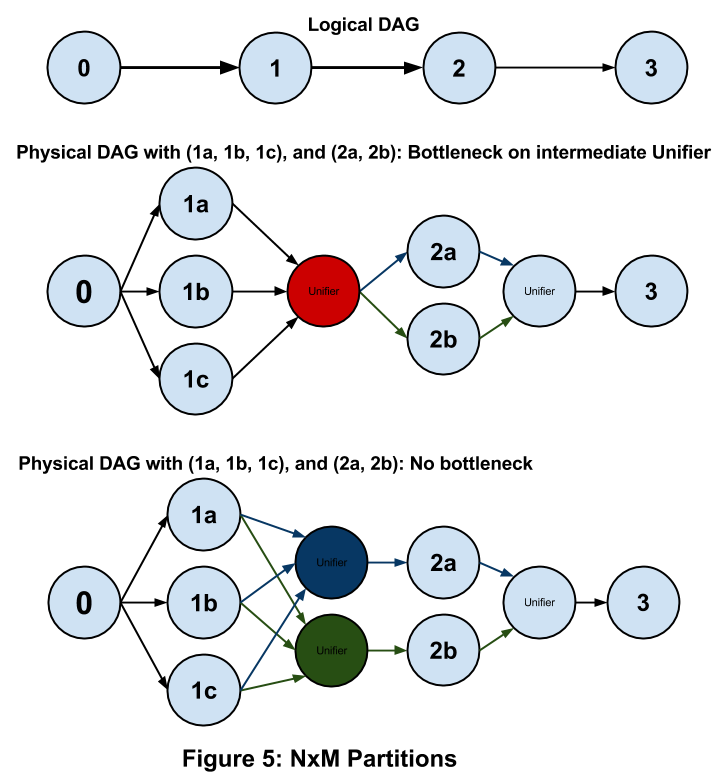
Parallel
In cases where all the downstream operators use the same partitioning scheme and the DAG is network bound an optimization called parallel partition is very effective. In such a scenario all the downstream operators are also partitioned to create computation flow per partition. This optimization is extremely efficient for network bound streams, In some cases this optimization would also apply for CPU or RAM bounded applications.
In Figure 6a, operator 1 is partitioned into 1a and 1b. Both the downstream operators 2 and 3 follow the same partition scheme as 1, however the network I/O between 1 and 2, and between 2 and 3 is high. Then users can decide to optimize using parallel partitions. This allows STRAM to completely skip the insertion of intermediate Unifier operators between 1 and 2 as well as between 2 and 3; a single unifier just before operator 4, is adequate by which time tuple flow volume is low.
Since operator 4 has sufficient resources to manage the combined output of multiple instances of operator 3, it need not be partitioned. A further optimization can be done by declaring operators 1, 2, and 3 as THREAD_LOCAL (intra-thread) or CONTAINER_LOCAL (intra-process) or NODE_LOCAL (intra-node). Parallel partition is not used by default, users have to specify it explicitly via an attribute of the input port (reader) of the stream as shown below.
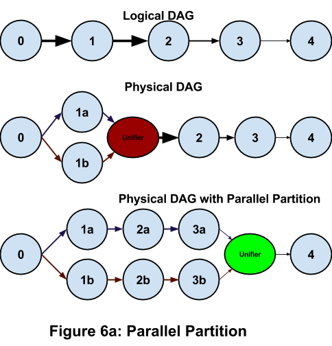
The following code shows an example of creating a parallel partition.
dag.addStream("DenormalizedUserId", idAssigner.userid, uniqUserCount.data);
dag.setInputPortAttribute(uniqUserCount.data, PortContext.PARTITION_PARALLEL, partitionParallel);
Parallel partitions can be used with other partitions, for example a parallel partition could be sticky key or load balanced.
Parallel Partitions with Streams Modes
Parallel partitions can be further optimized if the parallel partitions are combined with streams being in-line or in-node or in-rack mode. This is very powerful feature and should be used if operators have very high throughput within them and the outbound merge does an aggregation. For example in Figure 6b, if operator 3 significantly reduces the throughput, which usually is a reason to do parallel partition, then making the streams in-line or in-node within nodes 1->2 and 2->3 significantly impacts the performance.
CONTAINER_LOCAL stream has high bandwidth, and can manage to consume massive tuple count without taxing the NIC and networking stack. The downside is that all operators (1,2,3) in this case need to be able to fit within the resource limits of CPU and memory enforced on a Hadoop container. A way around this is to request RM to provide a big container. On a highly used Hadoop grid, getting a bigger container may be a problem, and operational complexities of managing a Hadoop cluster with different container sizes may be higher. If THREAD_LOCAL or CONTAINER_LOCAL streams are needed to get the throughput, increasing the partition count should be considered. In future STRAM may take this decision automatically. Unless there is a very bad skew and sticky key partitioning is in use, the approach to partition till each container has enough resources works well.
A NODE_LOCAL stream has lower bandwidth compared to a CONTAINER_LOCAL stream, but it works well with the RM in terms of respecting container size limits. A NODE_LOCAL parallel partition uses local loop back for streams and is much better than using NIC. Though NODE_LOCAL stream fits well with similar size containers, it does need RM to be able to deliver two containers on the same Hadoop node. On a heavily used Hadoop cluster, this may not always be possible. In future STRAM would do these trade-offs automatically at run-time.
A RACK_LOCAL stream has much lower bandwidth than NODE_LOCAL stream, as events go through the NIC. But it still is able to better manage SLA and latency. Moreover RM has much better ability to give a rack local container as opposed to the other two.
Parallel partitions with CONTAINER_LOCAL streams can be done by setting all the intermediate streams to CONTAINER_LOCAL. Parallel partitions with THREAD_LOCAL streams can be done by setting all the intermediate streams to THREAD_LOCAL. Platform supports the following via attributes.
- Parallel-Partition
- Parallel-Partition with THREAD_LOCAL stream
- Parallel-Partition with CONTAINER_LOCAL stream
- Parallel-Partition with NODE_LOCAL stream
- Parallel-Partition with RACK_LOCAL stream
These attributes would nevertheless be initial starting point and STRAM can improve on them at run time.
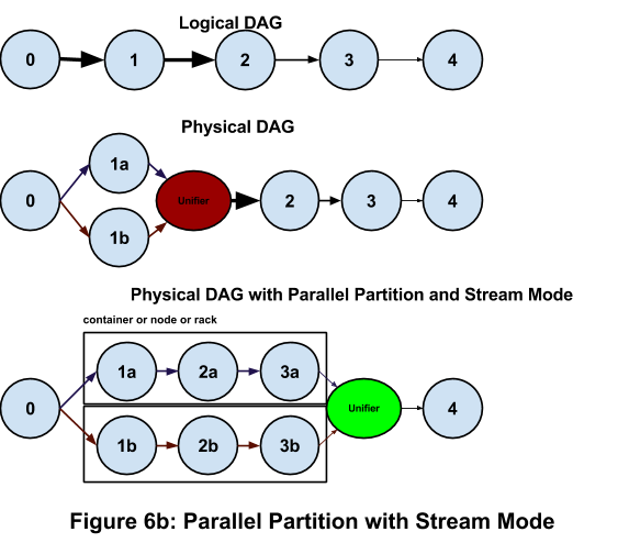
Skew Balancing Partition
Skew balancing partition is useful to manage skews in the stream that is load balanced using a sticky key. Incoming events may have a skew, and these may change depending on various factors like time of the day or other special circumstances. To manage the uneven load, users can set a limit on the ratio of maximum load on a partition to the minimum load on a partition. STRAM would use this to dynamically change the partitions. For example suppose there are 6 partitions, and the load happens to be distributed as follows: one with 40%, and the rest with 12% each. The ratio of maximum to minimum is 3.33. If the desired ratio is set to 2, STRAM would partition the first instance into two partitions, each with 20% load to bring the ratio down to the desired level. This will be tried repeatedly till partitions are balanced. The time period between each attempt is controlled via an attribute to avoid rebalancing too frequently. As mentioned earlier, dynamic operations include both splitting a partition as well as merging partitions with low load.
Figure 7 shows an example of skew balancing partition. An example of 3x1 paritition is shown. Let's say that skew balance is kept at “no partition to take up more than 50% load. If in runtime the load type changes to create a skew. For example, consider an application in the US that is processing a website clickstream. At night in the US, the majority of accesses come from the Far East, while in the daytime it comes from the Americas. Similarly, in the early morning, the majority of the accesses are from east coast of the US, with the skew shifting to the west coast as the day progresses. Assume operator 1 is partitioned into 1a, 1b, and 1c.
Let's see what happens if the logical operator 1 gets into a 20%, 20%, 60% skew as shown in Figure 7. This would trigger the skew balancing partition. One example of attaining balance is to merge 1a, and 1b to get 1a+1b in a single partition to take the load to 40%; then split 1c into two partitions 1ca and 1cb to get 30% on each of them. This way STRAM is able to get back to under 50% per partition. As a live 24x7 application, this kind of skew partitioning can be applied several times in a day. Skew-balancing at runtime is a critical feature for SLA compliance; it also enables cost savings. This partitioning scheme will be available in later release.
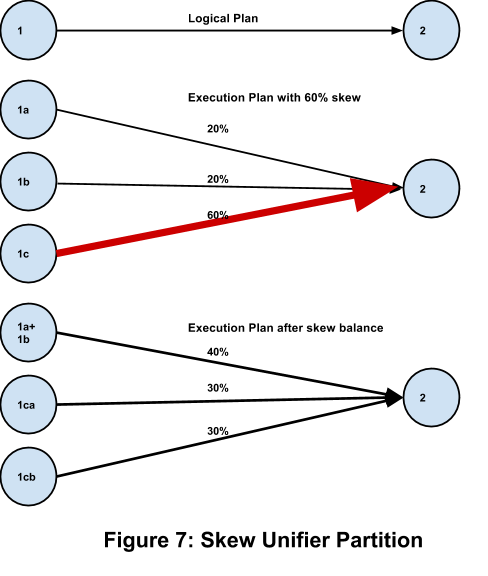
Skew Unifier Partition
In this section we would take a look at another way to balance the skew. This method is a little less disruptive, but is useful in aggregate operators. Let us take the same example as in Figure 7 with skew 20%, 20%, and 60%. To manage the load we could have either worked on rebalancing the partition, which involves a merge and split of partitions to get to a new distribution or by partitioning only the partition with the big skew. Since the best way to manage skew is to load balance, if possible, this scheme attempts to do so. The method is less useful than the others we discusse -- the main reason being that if the developer has chosen a sticky key partition to start with, it is unlikely that a load balancing scheme can help. Assuming that it is worthwhile to load balance, a special one-purpose unifier can be inserted for the skew partition. If the cause of resource bottleneck is not the I/O, specially the I/O into the downstream operator, but is the compute (memory, CPU) power of a partition, it makes sense to split the skew partition without having to change the in-bound I/O to the upstream operator.
To trigger this users can set a limit on the ratio of maximum load on a partition to the minimum load on a partition, and ask to use this scheme. STRAM would use this to load balance.The time period between each attempt is controlled via the same attribute to avoid rebalancing too frequently.
Figure 8 shows an example of skew load balancing partition with a dedicated unifier. The 20%, 20%, and 60% triggers the skew load balancing partition with an unifier. Partition 1c would be split into two and it would get its own dedicated unifier. Ideally these two additional partitions 1ca and 1cb will get 30% load. This way STRAM is able to get back to under 50% per partition. This scheme is very useful when the number of partitions is very high and we still have a bad skew.
In the steady state no physical partition is computing more than 30% of the load. Memory and CPU resources are thus well distributed. The unifier that was inserted has to handle 60% of the load, distributed more evenly, as opposed to the final unifier that had a 60% skew to manage at a much higher total load. This partitioning scheme will be available in later release.
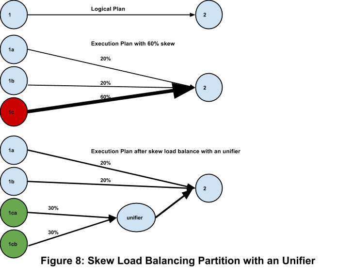
Cascading Unifier
Let's take the case of an upstream operator oprU that connects to a downstream operator oprD. Let's assume the application is set to scale oprU by load balancing. So this could be either Nx1 or NxM partitioning scheme. The upstream operator oprU scales by increasing N. An increase in the load triggers more resource needs (CPU, Memory, or I/O), which in turn triggers more containers and raises N, the downstream node may be impacted in a lot of situations. In this section we review a method to shield oprD from dynamic changes in the execution plan of oprU. On aggregate operators (Sum, Count, Max, Min, Range …) it is better to do load balanced partitioning to avoid impact of skew. This works very well as each partition emits tuples at the order of number of keys (range) in the incoming stream per application window. But as N grows the in-bound I/O to the unifier of oprU that runs in the container of oprD goes up proportionately as each upstream partition sends tuples of the order of unique keys (range). This means that the partitioning would not scale linearly. The platform has mechanisms to manage this and get the scale back to being linear.
Cascading unifiers are implemented by inserting a series of intermediate unifiers before the final unifier in the container of oprD. Since each unifier guarantees that the outbound I/O would be in order of the number of unique keys, the unifier in the oprD container can expect to achieve an upper limit on the inbound I/O. The problem is the same irrespective of the value of M (1 or more), wherein the amount of inbound I/O is proportional to N, not M. Figure 8 illustrates how cascading unifier works.
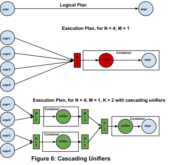
Figure 8 shows an example where a 4x1 partition with single unifier is split into three 2x1 partitions to enable the final unifier in oprD container to get an upper limit on inbound I/O. This is useful to ensure that network I/O to containers is within limits, or within a limit specified by users. The platform allows setting an upper limit of fan-in of the stream between oprU and oprD. Let's say that this is F (in the figure F=2). STRAM would plan N/F (let's call it N1) containers, each with one unifier. The inbound fan-in to these unifiers is F. If N1 > F, another level of unifiers would be inserted. Let's say at some point N/(F1*F2*...Fk) < F, where K is the level of unifiers. The outbound I/O of each unifier is guaranteed to be under F, specially the unifier for oprD. This ensures that the application scales linearly as the load grows. The downside is the additional latency imposed by each unifier level (a few milliseconds), but the SLA is maintained, and the application is able to run within the resource limits imposed by YARN. The value of F can be derived from any of the following
- I/O limit on containers to allow proper behavior in an multi-tenant environment
- Load on oprD instance
- Buffer server limits on fan-in, fan-out
- Size of reservoir buffer for inbound fan-in
A more intriguing optimization comes when cascading unifiers are combined with node-local execution plan, in which the bounds of two or more containers are used and much higher local loopback limits are leveraged. In general the first level fan-in limit (F1) and the last stage fan-in limit (Fk) need not be same. In fact a much open and better leveraged execution plan may indeed have F1 != F2 != … != Fk, as Fk determines the fan-in for oprD, while F1, … Fk-1 are fan-ins for unifier-only containers. The platform will have these schemes in later versions.
SLA
A Service Level Agreement translates to guaranteeing that the application would meet the requirements X% of the time. For example six sigma X is 99.99966%. For real-time streaming applications this translates to requirements for latency, throughput, uptime, data loss etc. and that in turn indirectly leads to various resource requirements, recovery mechanisms, etc. The platform is designed to handle these and features would be released in future as they get developed. At a top level, STRAM monitors throughput per operator, computes latency per operator, manages uptime and supports various recovery mechanisms to handle data loss. A lot of this decision making and algorithms will be customizable.
Fault Tolerance
Fault tolerance in the platform is defined as the ability to recognize the outage of any part of the application, get resources, re-initialize the failed operators, and re-compute the lost data. The default method is to bring the affected part of the DAG back to a known (checkpointed) state and recompute atomic micro batches from there on. Thus the default is at least once processing mode. An operator can be configured for at most once recovery, in which case the re-initialized operator starts from next available window; or for exactly once recovery, in which case the operator only recomputes the window it was processing when the outage happened.
State of the Application
The state of the application is traditionally defined as the state of all operators and streams at any given time. Monitoring state as every tuple is processed asynchronously in a distributed environment becomes a near impossible task, and cost paid to achieve it is very high. Consequently, in the platform, state is not saved per tuple, but rather at window boundaries. The platform treats windows as atomic micro batches. The state saving task is delegated by STRAM to the individual operator or container. This ensures that the bookkeeping cost is very low and works in a distributed way. Thus, the state of the application is defined as the collection of states of every operator and the set of all windows stored in the buffer server. This allows STRAM to rebuild any part of the application from the last saved state of the impacted operators and the windows retained by the buffer server. The state of an operator is intrinsically associated with a window id. Since operators can override the default checkpointing period, operators may save state at the end of different windows. This works because the buffer server saves all windows for as long as they are needed (state in the buffer server is purged once STRAM determines that it is not longer needed based on checkpointing in downstream operators).
Operators can be stateless or stateful. A stateless operator retains no data between windows. All results of all computations done in a window are emitted in that window. Variables in such an operator are either transient or are cleared by an end_window event. Such operators need no state restoration after an outage. A stateful operator retains data between windows and has data in checkpointed state. This data (state) is used for computation in future windows. Such an operator needs its state restored after an outage. By default the platform assumes the operator is stateful. In order to optimize recovery (skip processing related to state recovery) for a stateless operator, the operator needs to be declared as stateless to STRAM. Operators can explicitly mark themselves stateless via an annotation or an attribute.
Recovery mechanisms are explained later in this section. Operator developers have to ensure that there is no dependency on the order of tuples between two different streams. As mentioned earlier in this document, the platform guarantees in-order tuple delivery within a single stream, For operators with multiple input ports, a replay may result in a different relative order of tuples among the different input ports. If the output tuple computation is affected by this relative order, the operator may have to wait for the endWindow call (at which point it would have seen all the tuples from all input ports in the current window), perform order-dependent computations correctly and finally, emit results.
Checkpointing
STRAM provides checkpointing parameters to StreamingContainer during initialization. A checkpoint period is given to the containers that have the window generators. A control tuple is sent at the end of checkpoint interval. This tuple traverses through the data path via streams and triggers each StreamingContainer in the path to instrument a checkpoint of the operator that receives this tuple. This ensures that all the operators checkpoint at exactly the same window boundary (except in those cases where a different checkpoint interval was configured for an operator by the user).
The only delay is the latency of the control tuple to reach all the operators. Checkpoint is thus done between the endWindow call of a window and the beginWindow call of the next window. Since most operators are computing in parallel (with the exception of those connected by THREAD_LOCAL streams) they each checkpoint as and when they are ready to process the “checkpoint” control tuple. The asynchronous design of the platform means that there is no guarantee that two operators would checkpoint at exactly the same time, but there is a guarantee that by default they would checkpoint at the same window boundary. This feature also ensures that purge of old data can be efficiently done: Once the checkpoint window tuple is done traversing the DAG, the checkpoint state of the entire DAG increments to this window id at which point prior checkpoint data can be discarded.
In case of an operator that has an application window size that is larger than the size of the streaming window, the checkpointing by default still happens at same intervals as with other operators. To align checkpointing with application window boundary, the application developer should set the attribute “CHECKPOINT_WINDOW_COUNT” to “APPLICATION_WINDOW_COUNT”. This ensures that the checkpoint happens at the end of the application window and not within that window. Such operators now treat the application window as an atomic computation unit. The downside is that it does need the upstream buffer server to keep tuples for the entire application window.
If an operator is completely stateless, i.e. an outbound tuple is only emitted in the process call and only depends on the tuple of that call, there is no need to align checkpointing with application window end. If the operator is stateful only within a window, the operator developer should strongly consider checkpointing only on the application window boundary.
Checkpointing involves pausing an operator, serializing the state to persistent storage and then resuming the operator. Thus checkpointing has a latency cost that can negatively affect computational throughput; to minimize that impact, it is important to ensure that checkpointing is done with minimal required objects. This means, as mentioned earlier, all data that is not part of the operator state should be declared as transient so that it is not persisted.
An operator developer can also create a stateless operator (marked with the Stateless annotation). Stateless operators are not checkpointed. Obviously, in such an operator, computation should not depend on state from a previous window.
The serialized state of an operator is stored as a file, and is the state to which that the operator is restored if an outage happens before the next checkpoint. The id of the last completed window (per operator) is sent back to STRAM in the next heartbeat. The default implementation for serialization uses KRYO. Multiple past checkpoints are kept per operator. Depending on the downstream checkpoint, one of these are chosen for recovery. Checkpoints and buffer server state are purged once STRAM sees windows as fully processed in the DAG.
A complete recovery of an operator needs the operator to be created, its checkpointed state restored and then all the lost atomic windows replayed by the upstream buffer server(s). The above design keeps the bookkeeping cost low with quick catch up time. In the next section we will see how this simple abstraction allows applications to recover under different requirements.
Recovery Mechanisms
Recovery mechanism are ways to recover from a container (or an operator) outage. In this section we discuss a single container outage. Multiple container outages are handled as independent events. Recovery requires the upstream buffer server to replay windows and it would simply go one more level upstream if the immediate upstream container has also failed. If multiple operators are in a container (THREAD_LOCAL or CONTAINER_LOCAL stream) the container recovery treats each operator as an independent object when figuring out the recovery steps. Application developers can set any of the recovery mechanisms discussed below for node outage.
In general, the cost of recovery depends on the state of the operator and the recovery mechanism selected, while data loss tolerance is specified by the application. For example a data-loss tolerant application would prefer at most once recovery. All recovery mechanisms treat a streaming window as an atomic computation unit. In all three recovery mechanisms the new operator connects to the upstream buffer server and asks for data from a particular window onwards. Thus all recovery methods translate to deciding which atomic units to re-compute and which state the new operator resumes from. A partially computed micro-batch is always dropped. Such micro-batches are re-computed in at-least-once or exactly-once mode and skipped in at-most-once mode. The notiion of an atomic micro-batch is a critical guiding principle as it enables very low bookkeeping costs, high throughput, low recovery times, and high scalability. Within an application each operator can have its own recovery mechanism.
At Least Once
At least once recovery is the default recovery mechanism, i.e it is used when no mechanism is specified. In this method, the lost operator is brought back to its latest viable checkpointed state and the upstream buffer server is asked to replay all subsequent windows. There is no data loss in recovery. The viable checkpoint state is defined as the one whose window id is in the past as compared to all the checkpoints of all the downstream operators. All downstream operators are restarted at their checkpointed state. They ignore all incoming data that belongs to windows prior their checkpointed window. The lost windows are thus recomputed and the application catches up with live incoming data. This is called " at least once" because lost windows are recomputed. For example if the streaming window is 0.5 seconds and checkpointing is being done every 30 seconds, then upon node outage all windows since the last checkpoint (up to 60 windows) need to be re-processed. If the application can handle loss of data, then this is not the most optimal recovery mechanism.
In general for this recovery mode, the average time lag on a node outage is
= (CP/2*SW)*T + HC
where
- CP - Checkpointing period (default value is 30 seconds)
- SW - Streaming window period (default value is 0.5 seconds)
- T - Time taken to re-compute one lost window from data in memory
- HC - Time it takes to get a new Hadoop Container, or make do with the current ones
A lower CP is a trade off between cost of checkpointing and the need to have to use it in case of outage. Input adapters cannot use at-least-once recovery without the support from sources outside Hadoop. For an output adapter care may needed if the external system cannot handle re-write of the same data.
At Most Once
This recovery mechanism is for applications that can tolerate data-loss; they get the quickest recovery in return. The restarted node connects to the upstream buffer server, subscribing to data from the start of the next window. It then starts processing that window. The downstream operators ignore the lost windows and continue to process incoming data normally. Thus, this mechanism forces all downstream operators to follow.
For multiple inputs, the operator waits for all ports with the at-most-once attribute to get responses from their respective buffer servers. Then, the operator starts processing till the end window of the latest window id on each input port is reached. In this case the end window tuple is non-blocking till the common window id is reached. At this point the input ports are now properly synchronized. Upstream nodes reconnect under at most once paradigm in same way. For example, assume an operator has ports in1 and in2 and a checkpointed window of 95. Assume further that the buffer servers of operators upstream of in1 and in2 respond with window id 100 and 102 respectively. Then port in1 would continue to process till end window of 101, while port in2 will wait for in1 to catch up to 102. From then on, both ports process their tuples normally. So windows from 96 to 99are lost. Window 100 and 101 has only in1 active, and 102 onwards both ports are active. The other ports of upstream nodes would also catch up till 102in a similar fashion. This operator may not need to be checkpointed. Currently the option to not do checkpoint in such cases is not available.
In general, in this recovery mode, the average time lag on a node outage is
= SW/2 + HC
where
-
SW - Streaming window period (default value is 0.5 seconds)
-
HC - Time it takes to get a new Hadoop Container, or make do with the current ones
Exactly Once
This recovery mechanism is for applications that require no data-loss as well are no recomputation. Since a window is an atomic compute unit, exactly once applies to the window as a whole. In this recovery mode, the operator is brought back to the start of the window in which the outage happened and the window is recomputed. The window is considered closed when all the data computations are done and end window tuple is emitted. Exactly once requires every window to be checkpointed. From then on, the operator asks the upstream buffer server to send data from the last checkpoint. The upstream node behaves the same as in at-most-once recovery. Checkpointing after every streaming window is very costly, but users would most often do exactly once per application window; if the application window size is substantially larger than the streaming window size (which typically is the case) the cost of running an operator in this recovery mode may not be as high.
Speculative Execution
In future we looking at possibility of adding speculative execution for the applications. This would be enabled in multiple ways.
-
At an operator level: The upstream operator would emit to two copies. The downstream operator would receive from both copies and pick a winner. The winner (primary) would be picked in either of the following ways
- Statically as dictated by STRAM
- Dynamically based on whose tuple arrives first. This mode needs both copies to guarantee that the computation result would have identical functionality
-
At a sub-query level: A part of the application DAG would be run in parallel and all upstream operators would feed to two copies and all downstream operators would receive from both copies. The winners would again be picked in a static or dynamic manner
- Entire DAG: Another copy of the application would be run by STRAM and the winner would be decided outside the application. In this mode the output adapters would both be writing the result.
In all cases the two copies would run on different Hadoop nodes. Speculative execution is under development and is not yet available.
Dynamic Application Modifications
Dynamic application modifications are being worked on and most of the features discussed here are now available. The platform supports the ability to modify the DAG of the application as per inputs as well as set constraints, and will continue to provide abilities to deepen features based on this ability. All these changes have one thing in common and that is the application does not need to be restarted as STRAM will instrument the changes and the streaming will catch-up and continue.
Some examples are
- Dynamic Partitioning: Automatic changes in partitioning of computations to match constraints on a run time basis. Examples includes STRAM adding resource during spike in streams and returning them once spike is gone. Scale up and scale down is done automatically without human intervention.
- Modification via constraints: Attributes can be changed via Webservices and STRAM would adapt the execution plan to meet these. Examples include operations folks asking STRAM to reduce container count, or changing network resource restrictions.
- Modification via properties: Properties of operators can be changed in run time. This enables application developers to trigger a new behavior as need be. Examples include triggering an alert ON. The platform supports changes to any property of an operator that has a setter function defined.
- Modification of DAG structure: Operators and streams can be added to or removed from a running DAG, provided the code of the operator being added is already in the classpath of the running application master. This enables application developers to add or remove processing pipelines on the fly without having to restart the application.
- Query Insertion: Addition of sub-queries to currently running application. This query would take current streams as inputs and start computations as per their specs. Examples insertion of SQL-queries on live data streams, dynamic query submission and result from STRAM (not yet available).
Dynamic modifications to applications are foundational part of the platform. They enable users to build layers over the applications. Users can also save all the changes done since the application launch, and therefore predictably get the application to its current state. For details refer to Configuration Guide .
Demos
The source code for the demos is available in the open-source Apache Apex-Malhar repository. All of these do computations in real-time. Developers are encouraged to review them as they use various features of the platform and provide an opportunity for quick learning.